A vast range of natural phenomena are described by a Power Law relationship.¹ The following excerpt from reference [1] suffices for an appreciation of the power law's scope.

"The distribution of a wide variety of natural and man-made phenomena follow a power law, including frequencies of words in most languages, frequencies of family names, sizes of craters on the moon and of solar flares, the sizes of power outages, earthquakes, and wars, the popularity of books and music, and many other quantities."

A power law is any polynomial relationship exhibiting scale invariance as described below.
Most commonly one has

y = f(x) = a xk

(1)

where a is a constant and k is the scaling exponent. For our purposes the independent variable x is the number of highpointers, or climbers generally; and the dependent variable y is the corresponding value in the relevant records list.²

It is not obvious that climber numbers form the "natural" set of independent variables. It seems perfectly acceptable to also consider values in the relevant records list as the independent set; and climber numbers as depending on them. One of the seven lists studied is analyzed in this fashion.

An alternative to the above formulation is given by integrating (1) with respect to variable x from infinity to x₀,

y = g(x) = a xk+1 / (k+1)	(2a)
= A x p	(2b)

where A = a / (k+1) and p = k+1 and the 0 subscript has been suppressed.

Owing to the often small number of data points for a given narrow range in x-values, the probability density given by Equation (1) often varies wildly. To smooth over this effect, Equation (2b) is used in the detailed calculations, i.e. a cumulative probability distribution describing how many climbers have at least a specified cutoff value in the list.

Scale Invariance

A phenomenon exhibiting scale invariance has the property that multiplying the variable x by a constant factor causes only a proportionate scaling of the function itself, i.e. for Equation (1),

y = f(cx) = a (cx)k = ck f(x) .

(3)

Thus scaling by a constant c multiplies the original power law relation by the constant c^k. It follows that all power laws with a particular scaling exponent are equivalent up to constant factors, each being a scaled version of the others.

Taking the logarithm on both sides of Equation (2b),

ln y = ln A + p ln x .

(4)

Seven lists are selected as representive of both the county highpoint FRL ("Front Runner Lists") and the prominence-based lists available at peakbagger.com.

1. County highpoint Century Club, the list of highpointers
   with at least 100 county highpoints visited apiece.

   Figure 1 (Click for the actual graph.)

2. County highpoint home glob radius - radius of the largest circle, centered at the highpointer's home, such that no unclaimed county or part thereof lies within the circle.

   Figure 2 (Click for the actual graph.)

3. U.S.A. national forest highpoints, a list included because the author is unaware of anybody actively pursuing this list for its own sake.³ This lack of intention is important as discussed later.

   Figure 3 (Click for the actual graph.)

4. Worldwide 600+ meter prominences as climbed by members of peakbagger.com.⁴

   Figure 4 (Click for the actual graph.)

5. County highpoint state completions by person, the list of how many states have seen their respective county highpoints completely visited by specific individuals.⁵ The independent and dependent variables are reversed, i.e. cumulative highpointer counts are considered a function of how many states they minimally have completed.

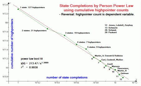
   Figure 5 (Click for the actual graph.)

6. County highpoint total area - the summed areas, in square miles, of all counties with visited highpoints for specific individuals.

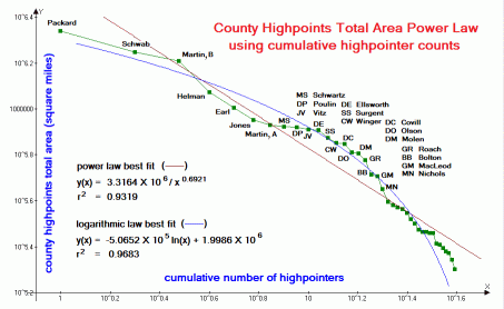
   Figure 6 (Click for the actual graph.)

7. Worldwide 1,500+ meter ("ultra") prominences as climbed by members of peakbagger.com.⁶

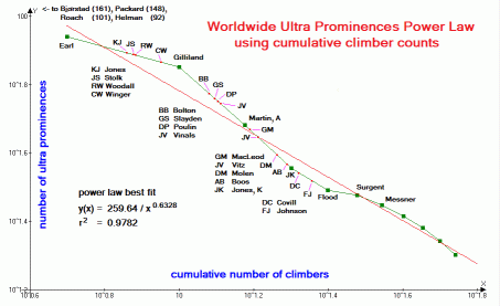
   Figure 7 (Click for the actual graph.)

Lists are graphed and analyzed using values from March 13 and 15, 2011. There is no reason to suspect that the analysis and/or interpretation qualitatively depend on the exact dates.

For each list the least-squares best-fit to numerous functional forms is obtained; including, in addition to a power law relationship the following other types:

General

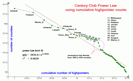
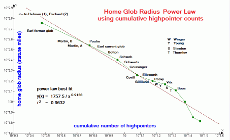
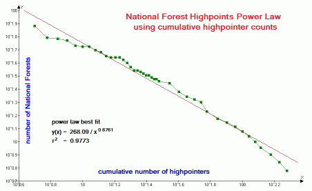
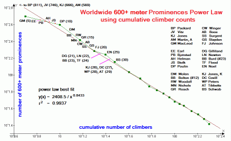
Examination of Figures 1-7 reveals that, in all cases a power law fit (straight line) qualitatively reproduces the data. In all cases the correlation coefficient r² exceeds 0.93 and with a mean value of 0.9687. For the worldwide 600+ meter prominence list (Figure 4) and state completions by person list (Figure 5) r² is remarkably close to the 1.00 value of a perfect correlation - 0.9937 and 0.9938 respectively.

With each data set, the power law fit, as measured by r² is superior to the fits using linear, hyperbolic, logarithmic and exponential functions.⁷ The sole exceptions (see below) are with the Century Club data (Figure 1) and total county area data (Figure 6), for which logarithmic fits yield higher r² values.

In the Century Club set (Figure 1) this arises from a single, anomalous low-density of highpointers in the 300-450 county range that, owing to the convexity it creates in the overall curve, is more closely matched by a logarithmic fit. Examination of previous Century Club listings shows no such anomaly, and it is anticipated to vanish once several highpointers with 200-300 counties enter that range.

In the total county area set (Figure 6) the best-fit to a logarithmic function is shown as a blue curve. It is a closer fit than the power law because of the peculiar shape of the graphed data: one that has a "bulge" from about 8 to 20 highpointers ("MS" to "MN"); followed by a rapid dropoff in total area which falls under the straight line. It is unknown whether these two sections (bulge and rapid descent) are reproducible phenomena that persist over time.

With reference to the Century Club data (Figure 1), counties in the eastern U.S.A. are generally easier to "acquire" than those in the mountainous western states, with several possible in a single waking cycle. Therefore eastern highpointers have an advantage amassing large county numbers. It would be instructive to perform separate analyses for eastern and western contingents.

However the most productive of this county highpointing species, currently Bob Schwab and Bob Packard, have globs that connect their eastern and western accomplishments - so confounding any attempt at assigning them to just the eastern or western group.⁸ Furthermore, the northeastern list of 300 counties has been completed by several people - and, as described below this makes the corresponding graph top-heavy and so incapable of supporting a power law relationship.

The home glob radius record set (Figure 2) contains the opposite effect - here, the large size of western counties provides an advantage to western county highpointers. Indeed, the first eight entries represent home globs in the western states. It would be interesting to perform a separate analysis for just "eastern globs".

Total county areas (Figure 6) also favor the western county highpointer, and for the same reason. However the same uber-highpointers noted above confound any attempt at categorizing highpointers into eastern and western subspecies for separate analyses.

U.S.A. national forest highpoints (Figure 3) and state completions by person (Figure 5) are discussed in later subsections.

⁷ For n data points it is possible to exactly fit a polynomial expression of degree n-1.
  Hence the n-degree polynomial fit is always superior, as measured by r², to the other
  functional forms tested. This is no consolation as the individual terms have little or no
  physical significance. Furthermore, in general it is preferable to fit data using the least
  possible number of parameters - and as achievable using the two-parameters of a
  power law relationship. When two parameters can describe dozens of data points
  it is likely that they have some useful physical interpretation.
⁸ In addition Bob Schwab's Midwestern USA accomplishments render it
  unsatisfactory to describe him as an "eastern" or a "western" county highpointer.

Validity of Fits

There are many ways to identify a power law relationship in data. Several of them are described in reference [1], including graphical methods (such as employed here), use of the cumulative distribution (also employed here), binning methods (which can result in undesired bias), and use of a maximum likelihood estimator to obtain a statistically unbiased power law exponent p of Equation (2b).

More important, though, is determining the validity of a presumed power law formulation in the first place. Demonstrating that data indeed follow a power law relation requires more than just fitting a model to the data. Alternative functional forms may appear to follow a power-law form for some extent - and yet, when the data is extended to its uppermost and/or lowermost bounds it may be found that scale invariance is not forthcoming.

Thus it is easily concluded from the total county area data of Figure 6 that a logarithmic law might exist, i.e.

y = a ln x + b

(5)

simply because the resulting curve-fit is slightly improved from a power law fit.

Another example is provided by the Century Club graph of Figure 1 wherein an anomalous low climber density (at 300-450 counties) results in a better fit using the logarithmic function. Both examples have been discussed in the previous subsection.

How is one to "prove" the truthfullness of an assumed functional form? How close must a straight line be for it to be called a valid formulation? Just this: What is the probability that seven of seven climbing record sets all appear to follow a power law relationship (0.93 < r² < 1.0) by sheer coincidence?

Choice of Independent Variable

It is "natural" to let the number of peaks climbed etc ... be a function of how many climbers have at least that value in their resumé. However it is equally valid to let the number of peaks be the independent variable, and the number of climbers be dependent on it.

This concept may seem unintuitive, yet results in certain favorable outcomes when graphing the data. It is certainly a valid concept, as seen by solving Equation (2b) for x in terms of y. There results a power law relationship with a straight line plot on double-logarithmic axes.

Thus in Figure 5 there is just one data point per given value of the independent variable, e.g. 73 highpointers with at least 2 completed states.

Were one to graph this state completions by person records list using highpointer count as the independent variable, there would be dozens of cumulative highpointer data points (x-coordinate) all with the same minimum number of completed states (y-coordinate). The resulting graph is both visually unappealing and makes it difficult to decide which data points to include - or which to exclude while differentially weighting the included points.⁹

⁹ Differential weighting seems reasonable: should every highpointer with a single
  state completion be individually accorded the same degree of importance as that one
  highpointer leading the pack with 29 states to his credit? Likely not.
  This issue is avoided by reversing the roles of list value and cumulative highpointer count.

Limiting Behavior

The asymptotic behavior of these climber-based graphs do NOT follow a power law. At the very "lower end" lie the vast majority of people having zero climbing accomplishments. There likely follows a small fraction with one summit that was reached - perhaps by chance in driving there. A smaller fraction still have two peaks to their credit. It is conceivable that this low-end climber count is described by a Poisson distribution.

At the "upper end" some lists have been "maxed-out" such that no "skinny tail" exists, i.e. county highpoint APEX peaks (20 maximum) and number of states in a glob (48 maximum).

Therefore climber's peak numbers etc... do not reflect true scale invariance; and as such the power law concept is limited in scope to a narrow range - and even then only for peak lists and records categories that have never been completed by any one person.

Climber Intention

Many climbers select peaks because they are on specific lists - with multiple list membership being a most attractive bargain for visiting their summits. Thus the author intentionally seeks ultra prominence mountains when traveling abroad to maximize the perceived benefit on a limited time budget. As a result, the number of ultra summits climbed is disproportionately represented relative to summits of lesser topographic prominence.

Does this penchant for specific summits alter the analysis? Examination of Figure 3 for U.S.A. national forest highpoints suggests not: nobody is currently pursuing this list for its own sake, with counts arising by happy coincidence from having climbed list members for entirely different reasons. Yet the graph closely follows the straight line indicative of a power law relationship.

Conclusion